Example 2: Inverse Design (NEW!)

In this example, we will design a nanomaterial withi a prescribed effective thermal conductivity tensor (diagonal components). To this end, we first get a BTE solver, specifically developed for inverse design

from openbte.inverse import bte

grid = 20

f = bte.get_solver(Kn=1, grid=grid,directions=[[1,0],[0,1]])

The function f takes the material density and gives the effective thermal conductivity tensor as well as its gradient wrt the material density. It is a differentiable function, i.e. it can be composed with arbitrary JAX functions to obtain end-to-end differentiability. This approach allows us to write down generic cost functions. In this case, we want to minimize \(||\kappa - \tilde{\kappa} ||\), where \(\tilde{\kappa}\) is the desired value

from jax import numpy as jnp

kd = jnp.array([0.3,0.2])
def objective(x):

     k,aux  = f(x)

     g  = jnp.linalg.norm(k-kd)

     return g,(k,aux)

The gradient is managed automatically. Finally, the optimization is done with

from openbte.inverse import matinverse as mi

L = 100 #nm
R = 30  #nm

x = mi.optimize(objective,grid = grid,L = L,R = R,min_porosity=0.05)

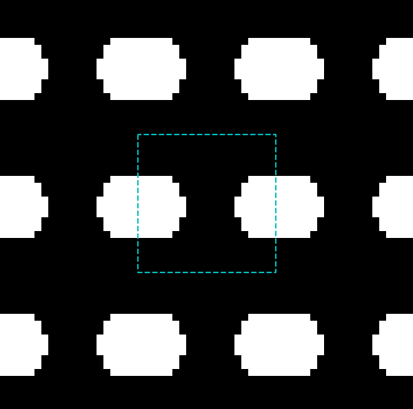
where R is the radius of the conic filter. Lastly, you can visualize the structure with

mi.plot(x)